Universidade Federal do Ceará
Grupo de Atenção Integral e Pesquisa em Acupuntura e Medicina Tradicional Chinesa – GAIPA UFC

ANOVA One Way;

ANOVA Two Way;

ANCOVA.

ANOVA Fatorial de medidas repitadas ou Mista;

ANCOVA;

MANOVA;

MANCOVA;

Modelo linear de efeitos mistos. (opção 2)

Kruskal-Walis;

Friedman.

Qui-Quadrado de Pearson (independência).

Exato de Fisher.

Alfa de Cronbach (α);

Coeficiente de Correlação Intraclasse (ICC);

Curva ROC;

Análise de Bland-Altman.

Estudo transversal

Ex. https://www.scielo.br/j/reben/a/WDRM3Wy3KNjxDYBCzxk4Ltm/?lang=pt

Os dados foram digitados em dupla entrada no programa Excel^®. Para verificar inconsistências, foram sobrepostos os bancos por meio do software Microsoft Excel 2016. Dados não recuperáveis foram registrados no banco como missing. A análise dos dados foi feita no programa Stata, versão 15.0. Inicialmente, foi realizado o teste de Kolmogorov-Smirnov com correção de Lilliefors para verificar a normalidade e as variáveis com p-valor>0,05 foram consideradas com distribuição normal ^{(Ghasemi A; Zahediasl S, 2012)}. Em seguida, foi feita a análise descritiva das variáveis sociodemográficas relacionadas à morbidade e à dor, expressas em frequência absoluta (n) e relativa (%), mediana, intervalo interquartil (IIQ) e valores de mínimo e máximo. Os domínios do WHOQOL-OLD foram ponderados com base em suas respectivas sintaxes e expressos em valores de média e desvio-padrão (DP).

Ensaio clínico

Ex. PMID: 34271271

We performed all the analyses in an intention-to-treat population, which included all patients who had undergone randomization and interventions. Descriptive statistics were applied to present the characteristics of each group with mean ± standard deviation, median (interquartile), or the number of cases (%).

Ex. PMID: 34271271

We performed all the analyses in an intention-to-treat population, which included all patients who had undergone randomization and interventions. Descriptive statistics were applied to present the characteristics of each group with mean ± standard deviation, median (interquartile), or the number of cases (%). All statistical analyses were conducted using Statistical Analysis System (SAS) version 9.2 (SAS Institute Inc., 2010).

Conversão de valores

Estimar a média e DP a partir da mediana e IQ <Clique aqui>

Estimar o DP a partir do erro padrão ou IC95% <Clique aqui>

Estimar o DP a partir do p-Valor e t-Valor <Clique aqui>.

Estimar o IC95% para médias e proporções <Clique aqui>

Combinar médias e DPs em um único grupo <https://www.statstodo.com/CombineMeansSDs.php>

Análise Estatística

Estatística no Excel

REAL STATISTICS USING EXCEL <https://www.real-statistics.com/>.

Suplementos <https://drive.google.com/file/d/19w1hJTiTG04uA3fXoyamZBVyPRwJEJtl/view?usp=sharing>.

Estatística no R e RStudio

Canal do Prof. Ronaldo Lima Jr. (UNB) <https://www.youtube.com/watch?v=sjX4rPfA_H0&list=PLzkA7H-mNfYhdbUe1e0FMpJDdLj1585zq>.

Tutoriais para análise estatística no SPSS

Análise descritiva e inferencial (testes de associação e comparação)  <Clique aqui>.

Análise testes de comparação <Clique aqui>. <Clique aqui>.

Análise testes de Regressão (linear e múltipla) <Clique aqui>.

Análise testes de Regressão (linear e logística) <Clique aqui>.

Análise testes de Validade e Confiabilidade <Clique aqui>.

Análise da pontuação do WHODAS 2.0 <Clique aqui>.

Tutorial para metanálise

Metanálise utilizado o RevMan <Clique aqui>.

ENSAIO CLÍNICO

Ex. PMID: 34271271

We performed all the analyses in an intention-to-treat population, which included all patients who had undergone randomization and interventions. Descriptive statistics were applied to present the characteristics of each group with mean ± standard deviation, median (interquartile), or the number of cases (%). Either analysis of variance or Chi-square test was used to reveal the baseline balance between groups, depending on the characteristics of the variables. The incidence of post- mastectomy chronic pain at 3 months and 6 months after surgery was compared with an unadjusted chi-square test. Logistic regression models with log links to estimate relative risk (RR) were used to assess RR with a 95% confidence interval (CI). Multiple comparisons between two groups were performed using the Chi-square partition method, in which the type I error was corrected to 0.0125 by the Bonferroni-adjusted method. Statistical significance was set at a two-tailed P-value of 0.05. In a post- hoc analysis, we assessed the heterogeneity of the treatment effect on post-mastectomy chronic pain at 6 months after surgery across study sites by testing for the treatment-by-site interaction. An interaction term <0.10 suggested potential treatment effect heterogeneity across sites. For missing data, analysis was performed according to a worst-case scenario. In particular, patients lost to follow-up in the two TEAS groups and those in the sham group were considered with and without pain, respectively. Stratified analysis by age, pre-existing pain at the surgery site, chemotherapy, radiotherapy, and endocrine therapy were performed using the Cochran-Mantel-Haensel test. All statistical analyses were conducted using Statistical Analysis System (SAS) version 9.2 (SAS Institute Inc., 2010).

Ex.: PMID: 12004740

Os dados dos participantes foram analisados por intenção de tratamento (intention to treat, ITT). Em casos de dropouts, o valor da última avaliação do participante foi replicado para o dado faltante (last observed carried forward, LOCF).

Ex.: PMID: 22968837

In order toaccount for missing data, all analyses were performedusing the ‘last observation carried forward’ method forintention-to-treat analysis. The level of significancewas set at p < 0.05, but when appropriate adjusted tothe 0.01 level to account for potential type I errors.

Ex. PMID: 39653805

The individuals included in the study, male or female, defined by chromosomal genotype, were randomized using a tool available on the internet (http://randomization.com), with the generation of a random sequence. Using the permuted block method, every individual was allocated to a single group, with 14 blocks of 6 each, totaling 84. In this way, they had the same probability of being drawn and allocated to one of the 3 study groups: traditional acupuncture (TA), laser acupuncture (LA), and sham laser acupuncture (S-LA). The researcher responsible for the randomization had no other role in this study.

Ex. PMID: 30356057
Patients were informed, both orally and in writing, that this study would distinguish two forms of interventions (APU and ACU)12, and about the possibility of 33% to be allocated to a control group, where they would receive the same anaesthetic care and attention by the study team as all other participants. Following written informed consent, patients were randomly assigned to either ACU, CON or APU by using the internet based randomization software RANDOULETTE® (Institute of Medical Information Sciences, Biometry and Epidemiology, Ludwig-Maximilians-University of Munich). Blinding of patients and assessors was ensured by using press needles & press plasters12. Patients in the control group could not be blinded.

FÓRUMULAS

N = tamanho da população.

n = tamanho da amostra.

δ = nível de confiança escolhido, expresso em número de Desvio Padrão (por convenção utiliza 1,96).

P =prevalência do fenômeno, ou percentagem (expresso em decimal).

Q = percentagem complementar, ou quociente (Q=1-P).

e = erro máximo permitido (por convenção se utiliza 3, 4 ou 5).

CÁLCULO AMOSTRAL PARA POPULAÇÃO FINITA

n = δ² x P x Q x N / e² (N-1) + (δ² x P x Q).

CÁLCULO AMOSTRAL PARA POPULAÇÃO INFINITA

n = δ² x P x Q / e².

• Conventional Rules.
  • “Because cross-validity formula estimates are primarily functions of sample size and the number of predictors, conventions have evolved that are based on the premise that with a large enough ratio of subjects to predictors, the sample regression coefficients will be reliable and will closely estimate the true population values (Miller & Kunce, 1973; Pedhazur & Schmelkin, 1991; Tabachnick & Fidell, 2001). For example, Stevens (2002) suggested a ratio of 15 subjects for each predictor (e.g., with 3 predictors 45 subjects are required) and Pedhazur and Schmelkin (1991) recommended N ≥ 30k, where k is the number of predictors. Others have provided rules that combine some minimum value with a subject-to-predictor ratio, including N ≥ 30 + 10k (Knapp & Campbell-Heider, 1989), N ≥ 50 + k (Harris, 1985), and N ≥ 50 + 8k (Green, 1991). Sawyer (1982) developed a formula where setting an inflation factor to a constant of 5% results in a sample size recommendation of N ≥ 10.8k + 11.8.”

Estudo transversal

O processo de amostragem foi estratificado por grupos para ser representativo para a população do estudo. A amostragem probabilística foi realizada em duas etapas, primeiramente por meio de setores censitárias e depois por domicílios, de acordo com as recomendações do Instituto Brasileiro de Geografia e Estatística (IBGE). Para o cálculo final da amostra, foram consideradas estimativa de prevalência de 50%, nível de confiança de 95%, erro máximo de 0,10 e o drawing effect de aproximadamente 2. O tamanho mínimo da amostra para o estudo foi de aproximadamente 400 participantes. A fim de maximizar a representatividade da amostra, 1.557 mulheres foram selecionadas aleatoriamente e entrevistadas.

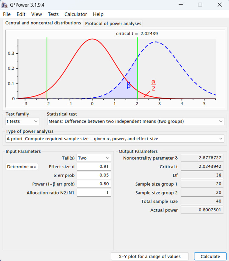
Ensaio clínico 

EX. PMID: 39804870

The sample size was calculated using G*Power software version 3.1.9.7, with a focus on achieving a robust estimate for detecting clinically meaningful changes. Specifically, a minimum clinically important difference (MCID) of 11.1 points, with a standard deviation (SD) of 3.8 points, was used based on established values for the primary outcome, the total Knee Injury and Osteoarthritis Outcome Score (KOOS) [24]. This estimation considered a power of 80%, an effect size of 0.2, a significance level of 5%, and an anticipated dropout rate of 20% [25, 26]. Consequently, the total calculated sample size was 50 participants, evenly divided into two groups of 25 participants each. KOOS was selected as the primary outcome measure for this study due to its comprehensive assessment of key domains relevant to KOA, including pain, symptoms, activities of daily living, sport and recreation, and quality of life [27]. The tool has been widely validated in populations with KOA and is sensitive to changes following interventions, making it an appropriate and robust measure for capturing patient-reported outcomes in this context [27].

Ex. PMID: 18601750

In calculating the sample size, a power of 90% and an α value of 5% were assumed, to detect a mean change in pain intensity, measured on the 100 mm visual analogue scale, of 32.3 mm between the initial and final values among the experimental group, and a mean reduction of 19.8 mm among the control group (standard deviation 31.9 mm). These assumptions require a sample size of 140 patients per group, in a design with two equal groups. We propose to recruit 400 patients in order to allow for a 30% drop out rate.

Ex. PMID: 22732720

A previous study reported a cumulative PONV incidence of 26% to 74% at 24 hours after surgery using prophylaxis with ondansetron and dexamethasone in patients after infratentorial craniotomy. Assuming an incidence of 40%, a sample size of 60 patients was determined by an a priori power analysis to provide an 80% power to be adequate to detect a 25% absolute reduction from 40% in the control group to 15% in the TEAS group at a= 0.05.

Ex. PMID: 34271271

The primary hypothesis was that TEAS would reduce chronic pain at 6 months after mastectomy, and combined acupoint stimulation would be more effective than single acupoint stimulation. We calculated that a sample size of 537 participants would have 80% power to detect a difference in the incidence of chronic pain at 6 months after mastectomy among the combined acupoints (25%), single acupoint group (30%), and sham-operated groups (40%), using two degrees of freedom chi-square test with a significance alpha level of 0.05. Considering a dropout rate of 5%, we defined a sample size of 576 participants.

Ex. PMID: 39653805

The sample size was calculated considering a difference of 1.5 points between groups, which would be a clinically relevant value for the outcome of neck pain intensity, as measured using the NRS [36], with an estimated standard deviation of 1.6 points, based on a clinical study about cervical pain [17]. The statistical power of 80% and a possible sample loss of 20% were adopted, considering dropouts for any reason. Therefore, 84 individuals were needed, with 28 in each group (TA, LA, and S-LA). The sample size was calculated using Minitab v.17 software (State College, PA, USA).

Ex. PMID: 30356057
The sample size of 75 patients was estimated on the basis of a supposed small to medium effect (Cohen’s d = 0.4) on post-operative recovery, an alpha-error of 5%, a power of 80% and a drop-out rate of 15% using G*Power (Version 3.1.3, University of Düsseldorf, Germany)11. The estimated time to recovery following gynaecologic laparoscopy in our clinic has been observed to range from 45 to 60 minutes, similar to published data resulting from mini cholecystectomy13. Shortening this time by 25% (i.e. 11 to 15 minutes) seems to be clinically meaningful14.

Ex. PMID: 40070890

• Cohen’s d = (Mean group B – Mean group A)/Pooled standard deviation.
• Pooled standard deviation = √((Standard deviation Group A² + Standard deviation Group B²)/2).
• Classificação do tamanho de efeito: 0.01-0.19 (muito pequeno); 0.20-0.49 (pequeno); 0.50-0.79 (moderado); 0.80-1.19 (grande); 1.20-1.99 (muito grande); >2.00 (enorme).

Ensaio clínico

Ex. PMID: 39653805

The magnitude of the intergroup difference was calculated using Cliff’s delta (ƍ) [Cliff N, 2014], with classification as not significant (ƍ < 0.147), weak (ƍ < 0.330), médium (ƍ < 0.474), or strong (ƍ ˃ 0.474) [Romano J, Coraggio JS, Kromrey J; 2006].

Ensaio clínico

Ex. PMID: 34271271

We performed all the analyses in an intention-to-treat population, which included all patients who had undergone randomization and interventions. Descriptive statistics were applied to present the characteristics of each group with mean ± standard deviation, median (interquartile), or the number of cases (%). Either analysis of variance or Chi-square test was used to reveal the baseline balance between groups, depending on the characteristics of the variables. The incidence of post- mastectomy chronic pain at 3 months and 6 months after surgery was compared with an unadjusted chi-square test. Logistic regression models with log links to estimate relative risk (RR) were used to assess RR with a 95% confidence interval (CI). Multiple comparisons between two groups were performed using the Chi-square partition method, in which the type I error was corrected to 0.0125 by the Bonferroni-adjusted method. Statistical significance was set at a two-tailed P-value of 0.05. In a post- hoc analysis, we assessed the heterogeneity of the treatment effect on post-mastectomy chronic pain at 6 months after surgery across study sites by testing for the treatment-by-site interaction. An interaction term <0.10 suggested potential treatment effect heterogeneity across sites. For missing data, analysis was performed according to a worst-case scenario. In particular, patients lost to follow-up in the two TEAS groups and those in the sham group were considered with and without pain, respectively. Stratified analysis by age, pre-existing pain at the surgery site, chemotherapy, radiotherapy, and endocrine therapy were performed using the Cochran-Mantel-Haensel test. All statistical analyses were conducted using Statistical Analysis System (SAS) version 9.2 (SAS Institute Inc., 2010).

Ex. PMID: 39653805

The Kolmogorov-Smirnov test was used to evaluate data normality. Data for the PPT and CPM, which presented normal distributions, were presented using means and standard deviations, together with the application of analysis of variance (ANOVA) for repeated measures, assuming a significance level of p<0.05. Data for the NRS, TS, and GPE, with non-normal distributions, were reported as pre- and post-treatment medians and Q3-Q1 interquartile ranges, difference scores (before– after), and the differences between them. The Kruskal-Wallis test was applied, with the posthoc Mann-Whitney U test for comparison between groups. The Mann-Whitney U test results were considered significant only for values below 0.0166 (Bonferroni correction: 0.05/3). The magnitude of the intergroup difference was calculated using Cliff’s delta (ƍ) [Cliff N, 2014], with classification as not significant (ƍ < 0.147), weak (ƍ < 0.330), médium (ƍ < 0.474), or strong (ƍ ˃ 0.474) [Romano J, Coraggio JS, Kromrey J; 2006]. Data processing employed the IBM SPSS Statistics v.19 for Windows software package.

PMID: 30356057

Data entry was carried out twice. Analysis was performed with the SPSS statistical software system (SPSS Inc., Chicago, IL; version 23.0). Fisher test was used to compare binary outcomes between the control and the intervention groups. Metric-variables were assessed for normal-distribution by Kolmogorov- Smirnov-Test. For normally distributed variables, the mean and standard deviation (SD) were calculated for descriptive analyses, and groups were compared by an analysis of variance (ANOVA). The unpaired t-Test was used for post-hoc pairwise comparisons. Influence of group x time of the state anxiety was assessed by ANOVA for repeated measures with group as between subject factor. In case of a non-normal distribution, non-parametric analyses were performed with descriptive statistics given as median (M) and interquartile-range (IQR). Kruskal-Wallis-Test was used for intergroup comparisons. Dunn’s Test was used for post-hoc pairwise group comparisons.

Ex. Paz MG da et al., 2021.

Análises bivariadas e múltiplas foram utilizadas para averiguar os fatores associados aos domínios da QV. Na análise bivariada realizou-se regressão linear simples para verificar associação entre as variáveis independentes e os domínios (variáveis dependentes). A seguir, variáveis com p-valor ≤ 0,20 na análise bivariada foram incluídas no modelo de regressão linear múltipla para ajuste das variáveis confundidoras (Schneider A et al., 2010). O método de entrada das variáveis foi feito em etapa única. A magnitude das associações foi apresentada em coeficiente de regressão não ajustado (β) com respectivos IC 95%. Os modelos foram avaliados e validados quanto aos seguintes pressupostos da regressão linear: (i) multicolinearidade pelo fator de inflação de variância (FIV) – considerou-se ausência de multicolinearidade FIV médio < 5,0 (Kim JH et al., 2019); normalidade dos resíduos pelo teste K-S, adotando valores de p do teste > 0,05 (Ghasemi A; Zahediasl S, 2012); (iii) homocedasticidade, avaliada pelo teste de Breusch-Pagan/Cook-Weisberg – a homocedasticidade dos modelos foi confirmada quando valor de p > 0,05 (Daye ZJ et al., 2012); e (iv) linearidade analisada pela visualização gráfica (26).